
Excel is widely known and used in the workplace as it’s several features allow us to find many uses for it such as creating Charts, reporting and visualizations, research, work scheduling and basic financial accounting.
However, we first have to know the basics when Excel before moving on to the more advanced functions it can offer. To begin, we will go over the layout of an Excel Worksheet: Cells, Rows, Columns and Tabs. Lastly, we will start learning what a formula is in Excel and it’s basic uses.
An Excel Worksheet is made up of several columns and rows that look like this:
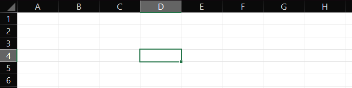
As you can see, this Worksheet has a bunch of empty white boxes called Cells. You can also see there is letters going across the cells at the top which are called Columns, which are labelled alphabetically. On the other hand, you can also see numbers to the left going downwards which are called Rows.
A Cell in Excel is an individual box within a Worksheet and contains text/numeric data. Each Cell has a name, which comes from the Column and Row the Cell sits on. If you’ve ever played the game Battleship, this should be familiar when referring to cells like “A7” and “C2”. Here is an example:
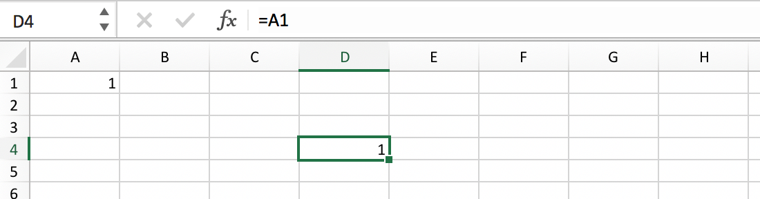
As you can see, there is an Excel spreadsheet with the number 1 in a certain cell, while the Column letters and Row numbers are displayed around it. By looking at what Column letter the 1 is contained with alongside the Row, you can see that this cell is called D4.
In an Excel document, you can have multiple Worksheets/Tabs. This can be very useful for storing multiple tables/records of data in an organised way rather than throwing them all into one. You can create another Tab in Excel by simply following the steps below:
Step 1- Click on the “plus” symbol
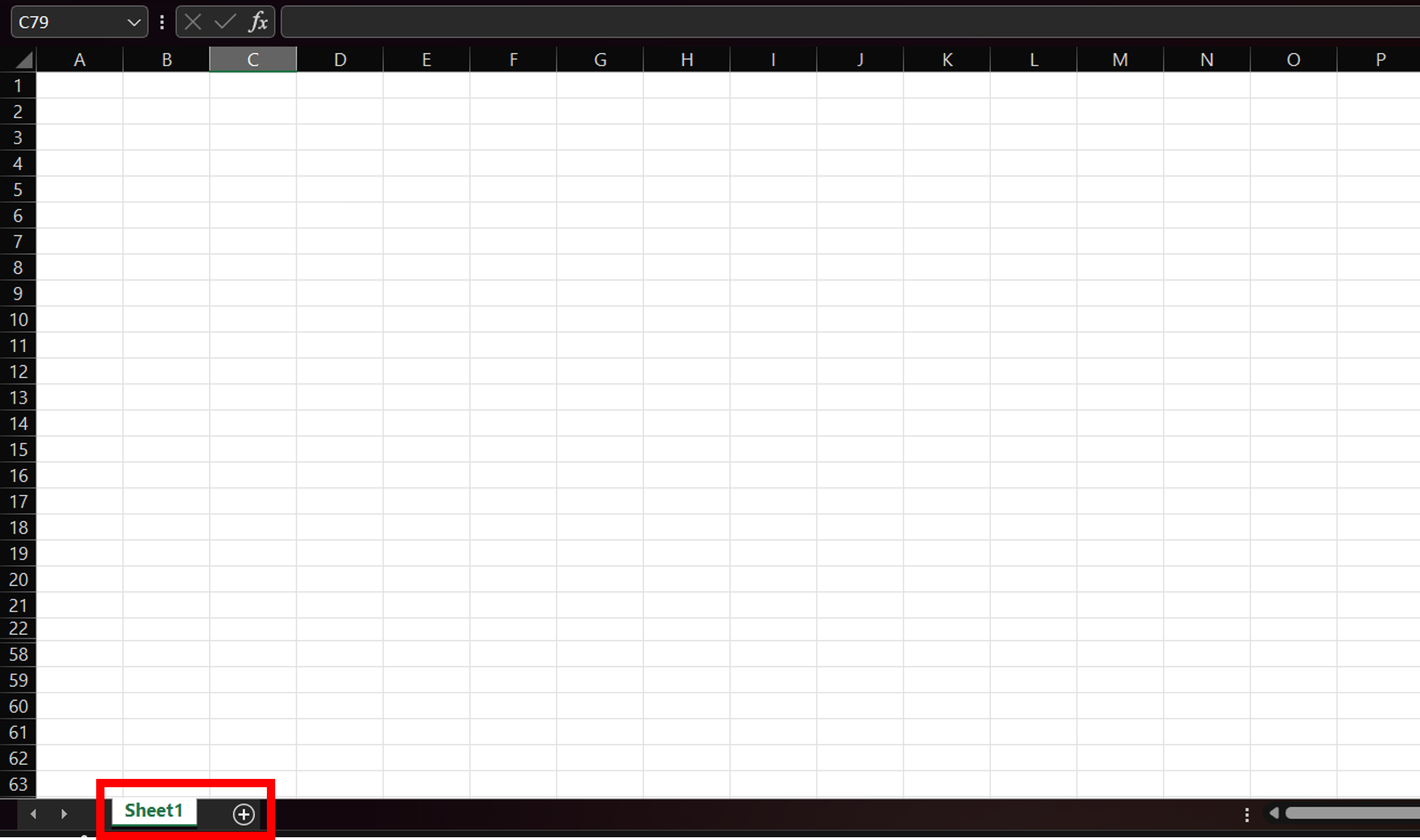
As shown in the red box, there is a Tab currently open called “Sheet1”, this is what every Excel document will look like when created. To the right of it however, is a plus symbol that will allow us to make another Tab when clicked on, as you can see here:
![]()
So now we know how to make another Tab, the last feature to learn is that every Tab can be named whatever you want. This is great for organisation rather than sifting through Sheet 1,2,3 you get it. To do this, simply right click on the Tab that you wish to rename and a drop down list of options should appear, the one you are looking for is called “Rename”. Once clicked, you should be able to then rename your Tab accordingly. like this:
![]()
One of Excel’s most unique features are formulas, but what actually are they? A formula is a manually inputted expression that operates on values in a range of cells. These formulas then output a result. At a basic level, Excel formulas enable you to perform calculations such as addition, subtraction, multiplication, and division.
When referring to a formula completing addition or subtraction you may think that these tasks are easy to do yourself and you’d be right! This is because for most of the time, Excel formulas offer convenience more than anything else.
When you have hundreds of accounting transactions on an Excel Worksheet, you could manually add up each and every one of them to get a total or you could use a basic function like “=SUM” to instantly calculate it. You could even change the numbers in the transactions and the total would automatically update! This is where the value of formulas shine, which moves us onto our next point, how do we actually make formulas in Excel?
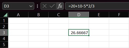
A formula always starts with an equal sign (=), which can be followed by numbers, math symbols (operators) like plus and minus or function. However, to multiply, you need to use the * symbol. You can then divide by using the / symbol. This means that we can make a basic mathematical equation without even using a function. An example of this can be seen below:
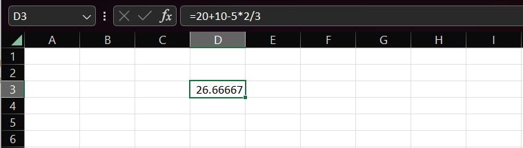
As you can see, there is a number in the cell D3. This is the result of the formula I’ve made right above it. Even though the formula is very simple in nature, when written down there it does tend to look a bit confusing so lets break it down.
First off, we put an equals sign (=) at the start of every formula. Then I have told the formula to add 20 and 10 together. After that, the formula will take 5 away from the total, multiply it by 2 and then divide it by 3.
Now you know what a formula is, you will need to know what functions are and how to use them to take full advantage of Excel’s features.
Functions are predefined formulas that perform calculations by using specific values, called arguments. These arguments have to be put in a particular order to work. The sheer amount of tasks you can complete with functions is why it’s complexity can range from simple to very advanced.
As there as so functions, Excel doesn’t expect us to remember all of them so they are all displayed when you click the formula button. You can see where it is on a Worksheet below:
In this image, you can see a small square button with the letters “fx” in it. When you click it, you should then see this:
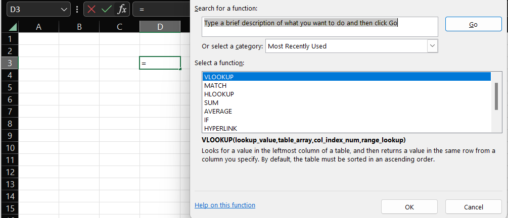
This pop-up contains a list of all the formulas in Excel, while also having a useful definition of what it does below. For this example, we will be using the formula called “SUM”. The purpose of this formula is to add numerical data up. Yet again, this formula offers convenience more than anything else, as adding up hundreds of payments in an accounting Worksheet for instance, would take much longer without using it. The only thing left to do now is to make this formula.
Like we’ve mentioned before, every formula starts with the equals sign (=). On top of that, if you are using a function, like we are now, then you have to put it straight after the equals. So if we put that together, our formula should start as “=SUM”.
Now we only need to input what we want to add together in the formula. You can do this manually by typing the names of cells in that you want to add up, however, I’ll show you a way that is much quicker.
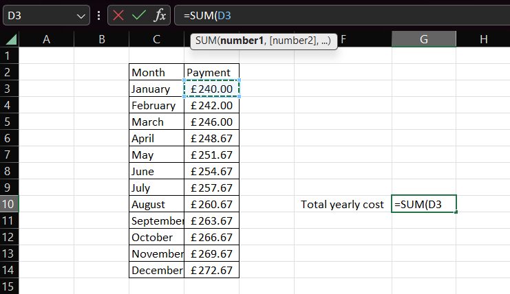
Firstly, you want to add a curved bracket after =SUM. This is because every function needs to have an opening and closing bracket at the start and end. Next, you want to click on the cell that you want to add up with, this should be the top or bottom cell in a list of data for convenience later on, as you can see, I’ve clicked on the cell at the top with January’s “payment” data. Now you are ready to click the same cell again then hold, dragging the mouse downwards to cover the rest of the data. If done correctly, the cells that you want to add up should look like this:
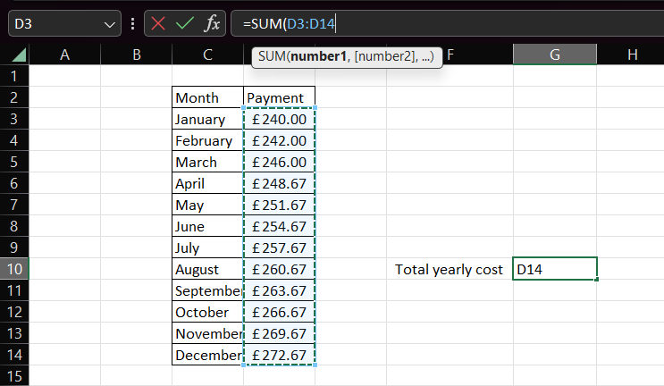
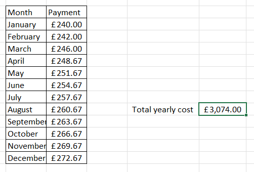
After this, you’ve reached the last step, all you need to do is simply add a closing bracket on the end of the formula and press enter. Well done! You’ve just created an Excel formula using a function. As you can see below, the formula has successfully added up all the monthly payments I’ve created on this Worksheet into a total:
For a start, if you’ve made it this far, congrats. In only one article we have learnt the basic layout of Excel, the key components of a formula, the definition and uses of a function and have made 2 examples of formulas. But why stop there? We are planning to release more and more knowledgebase material ranging from guides on choosing the right Managed IT Service Provider for you, to articles outlining the most common technical issues we solve for our customers daily.
So be sure to keep up to date with new knowledgebase article releases by singing up to our email listing below!